
Case Study – Internal Pilot – Machine Learning and Records Management March 20, 2018
Motivation
In 2017 State Archives NSW’s Digital Archives team began investigating the application of machine learning to records management. The first deliverable of this project was a research paper published on the FutureProof blog that explored the state of art (what the technology is capable of) and state of play (how it is being used in records management). One of the key findings of this report was that, although machine learning has potential to improve the classification and disposal of digital records, there has been very little adoption of the technology, particularly in New South Wales. In order to promote uptake we committed to a series of internal and external pilots to further explore and showcase machine learning for records management.
This case study documents an internal pilot that the Digital Archives team conducted in November and December 2017. The goal of this pilot was to apply off-the-shelf machine learning software to the problem of classifying a corpus of unstructured data against a retention and disposal authority. The results of this pilot were shared at the December 2017 Records Managers Forum.
Preliminary set-up
One of the constraints of the internal pilot was that we had limited resources: no budget and (very fortunately) an ICT graduate placement that had recent university experience in machine learning. So in identifying suitable technologies to use in the pilot we looked for low cost, off-the-shelf solutions. We quickly settled on scikit-learn: a free and open source machine-learning library for the Python programming language. This is a simple and accessible set of tools that includes pre-built classifiers and algorithms. It was fortunate that we had a machine with a big CPU, copious RAM, and SSDs to run the model on.
Method
Objective
The goal of the internal pilot was to test machine learning algorithms on a corpus of records that we had previously manually sentenced against a disposal authority. With what level of accuracy could we automatically match the corpus against the same disposal classes?
Corpus
The records that were chosen for the internal pilot had been transferred to the Digital State Archive in 2016 by a central government department. This corpus was unusual in that it contained a complete corporate folder structure extracted from Objective. The full corpus comprises 30 GB of data, in 7,561 folders, containing 42,653 files. At the point of transfer, no disposal rules had been applied to the files (ordinarily we require that only records required as State Archives are transferred to our custody). In a joint effort with the department we manually sentenced the corpus (at a folder level) against the General Retention and Disposal Authority Administrative Records (GA28). The result of this manual appraisal of the folders was a total of 12,369 files required as State archives.
The following options were considered for the internal pilot:
- to apply all “Required as State archive” classes from GA28 (75 in total). Folders that didn’t fit these classes would be unclassified
- to apply the subset of “Required as State archive” classes that had been manually identified in the corpus (23 in total). Folders that didn’t fit these classes would be excluded from the corpus
- to apply all of the GA28 classes (686 in total). To do a complete test of all folders
- to pre-treat the corpus by removing all folders which would be covered by NAP (Normal Administrative Practice) E.g. duplicates or non-official/ private records
The decision was made to pre-treat the corpus and remove all folders which would be covered by NAP (Normal Administrative Procedures) and to take the subset of 12,369 files that were identified as being “Required as State archives” which used only 23 classes of GA 28. Further preparation of the subset involved assigning the classification from the folder level at the level of the individual files. This was done manually.
Summary table
Break down of the corpus:
| Data set | Number of file contained |
| Complete corpus | 42653 |
| NAP (Normal Administrative Procedures) | 25643 |
| Corporate file plan | 17307 |
| Required as State Archives | 12369 |
| Required as State Archives and formats that could be text extracted – i.e. the usable sample set | 8784 |
Text Extraction and Classification steps
- Text Extraction
To be usable, the documents chosen for analysis need to be easily text extractable. This was to ensure performance and ease of conducting further text manipulation later in the project. Only 8,784 files of the 12,369 files which were classified as State archives were selected for use because their file types allowed simple text extraction.
After sorting the sample set, a Python program using various libraries was developed to extract text from the following file types: PDF, DOCX and DOC files.
The text that was extracted from documents was then placed within a single .csv file. The .csv file was divided into three columns: the file name (unique identifier), classification (GA 28 class), and lastly the text extract.
- Data cleaning
We took a very basic approach to data cleansing. The following concepts were utilised: remove document formatting, remove stop words, remove documents that are not required, and convert all letters to lower case.
- Text Vectorisation and Feature Extraction
Text vectorisation is the process of turning text into numerical feature vectors. A feature is unique quality that is being observed within a dataset and using these qualities we form an n-dimensional vector, which is used to represent each document. Text Vectorisation is necessary because machine learning and deep learning algorithms can’t work directly with text. It is essential to convert text into numerical values that the machine learning algorithm can understand and work with.
The methodology we used for text Vectorisation is termed the Bag-of-Words approach. This is a simple model that disregards the placements of words within documents but focuses on the frequency instead. This is done by considering each unique word as a feature. We then use this approach to represent any document as a representation of a fixed length of unique words known as the vocabulary of features. Each position for the unique word is filled by the count of the particular word appearing in that document, thus creating a document-term matrix which is a mathematical matrix that describes the frequency of terms that occur in a collection of documents
Example[1]
Suppose we have the vocabulary that includes the following:
Brown, dog, fox, jumped, lazy, over, quick, the, zebra
Then we are given an input document:
the quick brown fox jumped over the lazy dog
| Brown | Dog | Fox | Jumped | Lazy | Over | Quick | The | Zebra | |
| Document 1 | 1 | 1 | 1 | 1 | 1 | 1 | 1 | 2 | 0 |
This document term matrix shown above is the numerical representation of the given input document.
- Term Frequency Inverse Document Frequency (TF-IDF)
Having a document term matrix that uses counts is a good representation but a basic one. One of the biggest issues is that reoccurring words like “are” will have large count values that are not meaningful to the vector representations of documents. TF-IDF is an alternate method of calculating document feature values for a vector representation. TF-IDF works by calculating the term frequency (frequency of a particular word within a document) and then multiplying it by the Inverse document frequency (this helps decrease the rating of words that appear too frequently in the document set and favours unique/unusual words).
Therefore, once we had created a vocabulary and built the document term matrix (DTM) we applied the TF-IDF approach onto the DTM to increase the weighting of words that are unique to the documents themselves.
Example – Application on a Document-Term Matrix
Let’s say we have a document-term matrix with two documents in it and we want to put TF-IDF weighting on it.
| Brown | Dog | Fox | Jumped | Lazy | Over | Quick | The | Zebra | |
| Doc 1 | 1 | 1 | 1 | 1 | 1 | 1 | 1 | 2 | 0 |
| Doc 2 | 0 | 1 | 0 | 1 | 1 | 1 | 0 | 2 | 1 |
TF-IDF = Term Frequency * Inverse Document Frequency
Term Frequency = the number of times the word appears within a document.
Inverse Document Frequency = Log (Total number of documents / Number of documents having the particular word)
| Term Frequency | Inverse Document Frequency | TF-IDF | |||
| Doc 1 | Doc 2 | Doc 1 | Doc 2 | ||
| Brown | 1 | 0 | Log(2/1) = Log(2) | Log(2) | 0 |
| Dog | 1 | 1 | Log(2/2) = Log(0) = 0 | 0 | 0 |
| Fox | 1 | 0 | Log(2/1) = Log(2) | Log(2) | 0 |
| Jumped | 1 | 1 | Log(2/2) = Log(0) = 0 | 0 | 0 |
| Lazy | 1 | 1 | Log(2/2) = Log(0) = 0 | 0 | 0 |
| Over | 1 | 1 | Log(2/2) = Log(0) = 0 | 0 | 0 |
| Quick | 1 | 0 | Log(2/1) = Log(2) | Log(2) | 0 |
| The | 2 | 2 | Log(2/2) = Log(0) = 0 | 0 | 0 |
| Zebra | 0 | 1 | Log(2/1) = Log(2) | 0 | Log(2) |
After applying TF-IDF weighting it is clearly visible that words that are unique and provide greater meaning having higher weightings compared to those that don’t.
- Training and Test Split
The pilot used the standard ratio 75% training data to 25% testing data in its approach. To begin with we took 75% of the pre-classified “Required as State archive” content and used this data to train the algorithm to build the model. Once the training had been completed the same algorithm and model was used to process the 25% test set. This allows us to assess how accurately the model performs and determine a percentage of successful prediction. Our results are shown below.
- Machine learning algorithm overview
We used two machine learning algorithms to build our model: multinomial Naïve Bayes and the multi-layer perceptron. These algorithms were chosen as they are widely used for this type of application
- Multinomial Naïve Bayes
Multinomial Naïve Bayes is part of a family of simplistic probability based classifiers. The classifier is based on the Bayes theorem that involves the use of strong independent assumptions between features.
- Multi-Layer Perceptron
Multi-layer perceptron is a supervised learning algorithm that can learn as a non-linear function approximator for either classification or regression.
Statistical Analysis
To demonstrate the results of the internal pilot we have created a confusion matrix and summary result tables to display the comparison of the two algorithms used.
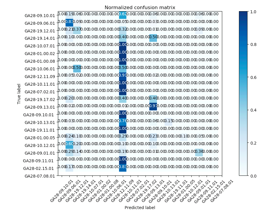
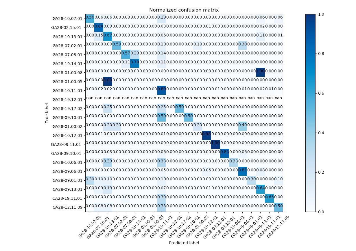
Confusion Matrix
A confusion matrix is a table that summarizes how successfully a classification model’s predictions were i.e. the correlation between the actual label and the model’s classification. One axis of a confusion matrix is the label that the model predicted, and the other axis is the actual label. The size of the table on both axes represents the number of classes. Note: The confusion matrices presented below are representative but aren’t the exact ones used to determine the results.
Confusion matrices contain sufficient information to calculate a variety of performance metrics, including precision and recall. Precision identifies the frequency with which a model was correct when predicting the positive class and recall answers the following question: out of all the possible positive labels, how many did the model correctly identify?
Multinomial Naïve Bayes
| Pre Data Cleaning | Cleaned Data |
| Features – 5,000
Best Accuracy: 65.4% F1 Score: 0.624 Training Time: 109 ms |
Features – 5,000
Best Accuracy: 69% F1 Score: 0.648 Training Time: 108 ms |
| Features – 10,000
Accuracy: 64% F1 Score:0.622 Training Time: 111 ms |
Features – 10,000
Accuracy: 68% F1 Score: 0.638 Training Time: 109 ms |
Multi-Layer Perceptron
| Pre Data Cleaning | Cleaned Data |
| Features – 5,000,
Accuracy: 77% F1 Score: 0.767 Training Time: 2 min 23s |
Features – 5,000
Accuracy: 82.7% F1 Score: 0.812 Training Time: 2 min 43s |
| Features – 10,000
Accuracy: 78% F1 Score: 0.777 Training Time: 3 min 28s |
Features – 10,000
Accuracy: 84% F1 Score: 0.835 Training Time: 4 min 02s |
Key Description
F1 Score[2]: is a measure of the models accuracy – It considers both the precision p and the recall r of the test to compute the score
Results
The pilot results have given us some pleasing statistics with a maximum of 84% successful hit rate using the Multi-layer Perceptron algorithm. The pilot gave us the opportunity to compare two algorithms and assess how both un-cleaned and cleaned data performed with those algorithms. The results demonstrate that this technology is capable of assisting with the classification and disposal of unclassified unstructured data.
Discussions
The following points provide considerations, limitations and the possible anticipation of the use of machine learning for records management:
- Any error made on the training data during sentencing will only increase in the model over time. This would also apply to any intentional bias created in the training data.
- The need for a large training set of classified data to achieve results over the test data.
- Using cloud services and understanding all the terms of services before using them is very important especially around issues of personal privacy of individuals and legal ownership of the data being stored.
- The corpus used was manually sentenced at folder level with only a sampling of individual documents whereas the model was able to sentence directly as document level in a much timelier manner.
- Having enough available computational volume on local machines to process the model.
- Exceptional results from only around 100 lines of code, having enough expertise and using the correct algorithm.
- Could we build a GA28 Machine Learning Black Box to help agencies manage administrative records?
- Do we know what the sentencing success rate was in the paper paradigm with manual human sentencing and how would that compare with the machine learning technologies?
I would like to thank and acknowledge the work of Malay Sharma (ICT Graduate) who was on a rotational placement just at the right time.
[1] https://stackoverflow.com/questions/17053459/how-to-transform-a-text-to-vector (Accessed on 1/12/2017)
[2] https://adamyedidia.files.wordpress.com/2014/11/f_score.pdf (Accessed on 5/12/2017)

Very interesting post especially for those not familar with some common methods in text classification.
For those already familar with text classification it would be even of more interest when the labeled training and test data set could be made available to interesting parties. Though many data sets are available on Kaggle and other ressources for structured data, there are only few pre-labeled sets for text and – as far as I know – no labled set which had been applied to records management. Thus, it would be great if you could share this data set (public or by NDA) so that other data scientiest could apply their expertise as well.
The missing point in ML and records management are data sets, not technology.
Best regards,
Gregor Joeris from SER (a software vendor of ECM and eletronic archives applying ML to content analytics)
Thank you for your comments Gregor. You are completely right & this is something we have discovered in our own investigations in this area: in order to make progress you really do need pre-labelled data in order to build the models. Unfortunately in this case we are unable to share the dataset as it contains government records that are closed until 2044. We’re engaging with NSW government agencies at the moment to develop further pilots and we will keep our eyes open for labelled material that could be shared as an open data set. Of course we’re happy to share the code from our experiment and as we make further progress we will continue to share our findings. All the best, Glen
Is the code you developed available (not dataset) on github – I couldn’t find the link
We will be publishing the code in the next post. Watch this space!